Variance is one of the building blocks of statistics. It measures how spread out a set of numbers are expected to be from their mean. The formal definition is pretty intuitive: Let $x$ be an array of all possible data points of interest for the whole population and $n$ the total number of data points. Variance over that population is then formally defined as follows:

$\sigma_x^2 = \frac{1}{n}\sum_{i=1}^n (x_i - \text{\={x}})^2$

You may have previously encountered this formula with one subtle difference: dividing by $n-1$. We divide by $n-1$ when we estimate the variance of the population from a given sample and by $n$ if we have population data. This is called Bessel’s correction^[1]. For the remainder of this post, we assume to be dealing with the whole population.

Many programming languages already provide with the standard library functions for the calculation of summary statistics; variance included. Here we’ll be playing with Python.

One implementation of a function to calculate variance could look like this:

def sigma2(x):
    n = len(x)
    mean = sum(x) / n
    return sum(x_i - mean)**2 for x_i in x) / n

Notice how here we need to iterate the array $x$ twice; first to find the mean, and then to find the sum of squares of the difference of each data point from the mean.

If we go back to the formal definition of the variance, with a bit of tweaking, we can compute it in one iteration, hopefully shaving off some time.

$\sigma_x^2 = \frac{1}{n} \sum_{i=1}^n (x_i - \overline{x})^2$

$= \frac{1}{n} \sum_{i=1}^n (x_i^2 - 2\overline{x}x_i + \overline{x}^2 )$

$= \frac{1}{n} \sum_{i=1}^n x_i^2 - \frac{2\overline{x}}{n}\sum_{i=1}^n x_i + \frac{n\overline{x}^2}{n}$

$= \frac{1}{n} \sum_{i=1}^n x_i^2 - 2\overline{x}^2 + \overline{x}^2$

$= \Large \lbrack \normalsize\frac{1}{n}\sum_{i=1}^n x_i^2 \Large \rbrack \normalsize - \overline{x}^2$

There are two parts to the derived formula:

• Sum of squares of all $x_i \in x$ divided by length of $x$.
• Mean squared of $x$.

We can calculate both in a single iteration. The implementation could be something like this:

def sigma1(x):
    n = len(x)
    mean = sum(x) / n
    sum_of_squares = 0
    for x_i in x:
        sum_of_squares += x_i * x_i
    return sum_of_squares / n - mean * mean

To compare the sigma1 implementation against the standard library statistics.pvariance. let’s make a list of 1 million random numbers from 0 to 1 and time how long it takes each function.

v = [random() for _ in range(1000000)]

Standard Library:

%timeit statistics.pvariance(v)
3.14 s ± 25.7 ms per loop (mean ± std. dev. of 7 runs, 1 loop each)

Single Iteration:

%timeit sigma1(v)
50 ms ± 870 µs per loop (mean ± std. dev. of 7 runs, 10 loops each)

sigma1 is ~63 times faster.

Alright, seems great but there’s an issue. The formula we derived to calculate the variance in a single iteration is not new. It’s often referred to as the computational formula for variance and it is subject to “catastrophic” cancellation effects when using floating point arithmetic with limited precision ^[2]. In fact, in the standard implementation of the Python language there’s a nice cautionary comment left:

Under no circumstances use the so-called “computational formula for variance”, as that is only suitable for hand calculations with a small amount of low-precision data. It has terrible numeric properties ^[3]

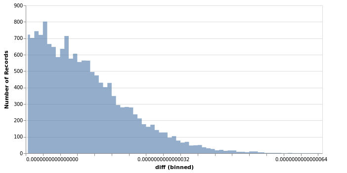
So just for fun, let’s check how big the discrepancies in output between statistics.pvariance and sigma1 are. Let’s run both 10k times on a list with 10k random numbers between 0 and 1.

The maximum difference observed is $6.86\mathrm{e}{-15}$. For many applications, this difference should be tolerable, but maybe enough to help a few needy researchers find the extra bit of significance to get their papers published.

Finally, let’s see why rolling own implementations of stuff is often unnecessary and and sometimes a bad idea. Let’s try Numpy^[4] - a scientific computing library for Python, written mostly in C. Let’s try numpy.var on the same setup:

%timeit numpy.var(v)
30.4 ms ± 313 µs per loop (mean ± std. dev. of 7 runs, 10 loops each)

This is ~1.6 times faster than sigma1, and ~103 times faster than the standard library implementation. The difference in output between statistics.pvariance and the numpy implementation is also slightly better compared to the differences we saw earlier with sigma1, the worst case here being $2.77\mathrm{e}{-17}$.

NOTE: This is not an exhaustive test setup to study the differences between these implementations.

---

1. Bessel’s Correction - Wikipedia ↩︎

2. Algebraic formula for the variance - Wikipedia ↩︎

3. Statistics Module Python Source ↩︎

4. Numpy - Homepage ↩︎