Residential segregation - a simulation

“People get separated along many lines and in many ways. There is segregation by sex, age, income, language, religion, color, taste, comparative advantage and the accidents of historical location. Some segregation results from the practices of organizations; some is deliberately organized; and some results from the interplay of individual choices that discriminate. Some of it results from specialized communication systems, like different languages. And some segregation is a corollary of other modes of segregation: residence is correlated with job location and transport.” Dynamic Models of Segregation ^[1] - Thomas C. Schelling, 1969

The main motivation for the paper was the study of the observed racial residential segregation in the United States. Schelling presented a model of segregation, in which individuals had no strong preferences against members of other groups, yet almost invariably resulted in segregation. Schelling writes:

The lines dividing the individually motivated, the collectively enforced, and the economically induced segregation are not clear lines at all. … This paper, then, is about those mechanisms that translate unorganized individual behaviour into collective results.

Let’s look at the model. Assume there’s a grid, where each cell is occupied by a person. Each person is a member of one group. The neighboring cells define the neighborhood. Each person is “happy” as long as at least some percentage of the neighbors belong to the same group they do. If a person is not happy, it moves to another location where they would be happy. This is a very simplified representation of the model, but a good enough one to get a feel for it.

When I first came across the paper, it reminded me of Conway’s Game of Life ^[2], in which simple rules, given a particular initial configuration would result in arbitrarily complex emergent patterns. Schelling’s model was not like that. With equally simple rules (albeit quite different), it seemed to have the propensity to converge in the segregation of groups.

Figure 1: Original illustrations from Dynamic Segregation Models - Thomas C. Schelling 1969

Half a century later, the same segregation that pushed Schelling to study the issue, is still visible ^[3]. Residential segregation is not limited to race. It can be observed with education, income and many other social facets.

In this blog post, we will get into more details of the model, build a simulator where we can study collective patters that emerge from individual behaviour. We’ll look at different model parameters, and try to figure out what parameters lead to integration or segregation. Hereafter: people -> population, person -> agent.

Simulation parameters and assumptions

There are 5 variables in the Linear Model Schelling opens the paper with:

Neighborhood (size)	The `k` nearest neighbors.
Similarity preference	Demanded percentage of one's own group in a neighborhood.
Population composition	Number of agents and percentage of the total population each group represents.
Initial configuration	The instantiation of the population (agent locations).
Rules governing movement	How often can an agent move, what's the cost function (i.e. prioritize for closeness) etc.

We’ll start with a population that is exhaustively divided into two groups, and every agent’s membership is permanent and recognizable. Each agent has a particular location at a given moment. The preferences of a group propagate to all of its agents. Each agent has then a preference to live in a neighborhood where at least some minimum fraction of neighbors are part of the same group. Throughout this simulation agent locations at the beginning will be drawn randomly from a uniform distribution (i.e. we expect agents to occupy uniformly the whole map or grid). Therefore Initial Configuration will remain constant.

Implementation: first round

We start by extracting the parameters that enable us to define a population and the preferences of the agents. We store these parameters in the variable config. This takes care of neighborhood size, similarity preference and the population composition.

config = {
    # size of population
    "agents": 10000,

    # similarity preference
    "similarity": 0.5,

    # neighborhood size
    "neighbors": 100,

    # population composition (defining groups)
    "groups": {
        "Group 1": {
            "type": "Group 1",
            # percentage of population
            "ratio": 0.5,
            "color": "#ff745c"
        },
        "Group 2": {
            "type": "Group 2",
            "ratio": 0.5,
            "color": "#c2bebe"
        },
    },
}

Then we need to generate a population from the config we defined earlier, as well as provide an original configuration for the simulation. To do this, let’s represent each agent by a numpy record array with three attributes:

agent = <x, y, group>

x, y determine the location of the agent in the map (cartesian plan) and group to denote the membership of the agent.

import numpy as np

def generate_population(config):
    # Load groups from config (`prob` is the % of the population
    # the group represents).
    groups, prob = zip(
        *sorted(
            [
                (g["type"], g["ratio"])
                for g in list(config["groups"].values())
            ],
            key=lambda x: x[1],
        )
    )
    agents = []
    # randomly spawn agents in different locations, and assign
    # to a group with a given probability (to approximate
    # a desired group size)
    for _ in range(config["agents"]):
        x = np.random.uniform(0, 1)
        y = np.random.uniform(0, 1)
        agents.append((x, y, np.random.choice(groups, p=prob)))

    # represent population as a record array
    # (convenient data structure)
    return np.rec.array(
        agents,
        dtype=[("x", "f"), ("y", "f"), ("group", "<U8")],
    )

At the beginning each agent is assigned a random location. The simulation will be iterative, in the sense that each round every unhappy agent will be given a chance to relocate.

In this first attempt, each agent will look at the neighboring 100 agents, and if the similarity preference is not satisfied the agent will, again, randomly be spawned at another location. The randomness in the way we define rules governing movement may appear “worrisome” for at least two reasons: Firstly, it does not reflect reality. Agents in real life will have information on the distribution and clustering of groups (e.g. Manhattan is where a lot of rich people live), and are expected to inform their decisions with it. Secondly, we may not get the simulation to converge into a stable equilibrium where all agents are happy. However for many configurations, you’ll observe segregation taking place nevertheless. Interestingly, Schelling’s restriction that one group is a minority, does not need to be imposed.

Anyway, here’s an implementation of the iteration-based simulation we described. Feel free to gloss over it, we’ll change it again later.

from collections import Counter
from sklearn.neighbors import KDTree

# will link to at the end (not important for now)
import plotting

def simulation(plot_folder):
    population = generate_population(config)

    stable = False
    iterations = 0

    while not stable and iterations < 100:
        locations = np.array(list(zip(population.x, population.y)))
        kdtree = KDTree(locations, leaf_size=100)

        agents_relocating = 0
        for agent in population:
            dist, idx = kdtree.query(
                [(agent.x, agent.y)],
                k=config["neighbors"]
            )
            neighborhood = Counter(population[idx[0]].group)

            # Check if agent needs to relocate
            observed_similarity = (
                neighborhood[agent.group]
                / sum(neighborhood.values()
            )
            if observed_similarity < config["similarity"]:
                agent.x = np.random.uniform(0, 1)
                agent.y = np.random.uniform(0, 1)
                agents_relocating += 1

        iterations += 1
        if agents_relocating < 5:
            stable = True

        # Produces a plot of the state at a given iteration
        plotting.population_scatter(
            population,
            iteration=iterations,
            folder=plot_folder,
            config=config
        )

In a nutshell, we instantiate a population, then keep iterating until either the population is stable (in the sense that it has reached an equilibrium) where agents have settled given their similarity preference, or there have been at most 100 iterations. The latter is merely there to guarantee the program terminates.

For each iteration, we build a k-d tree^[4] which we use to perform nearest-neighbor search over a neighborhood. Then, for each agent, we query the neighborhood to see the distribution of groups in that space, using which the agent decides whether or not to relocate.

Simulation 1: no minority

Let’s first look at a population of 10,000 agents. Each group makes half the population. Each agent prefers to have at least 50% of their neighbors belong to the same group they do.

Neighborhood size	100
Similarity preference	0.5
Population composition	10000 agents, 2 groups of equal size
Rules governing movement	If similarity preference not met, randomly relocate

Worth repeating, each agent wants to be in a neighborhood where they are not in minority.

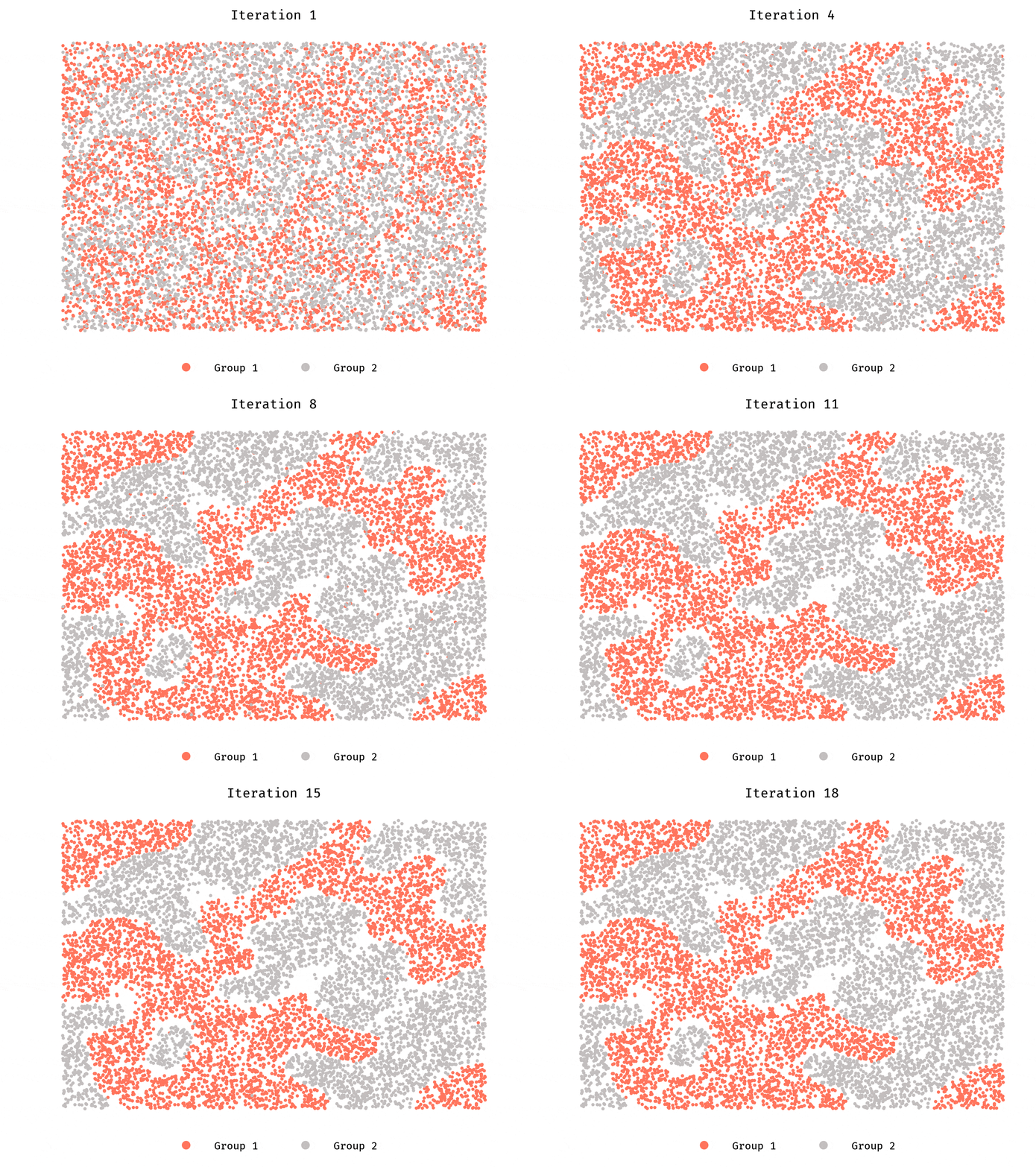
Figure 2: Population of 10k, equally represented by two groups, each of which prefers at least 50% of their neighbors to be from their own group

We see clusters forming very quickly, until they reach a stable equilibrium. Stable and desirable, however, are different things. Segregation is rampant.

Simulation 2: minority, looser similarity preference

Neighborhood size	100
Similarity preference	0.333
Population composition	10000 agents, 2 groups (30% and 70% of population)
Rules governing movement	If similarity preference not met, randomly relocate

This round we continue to simulate a population of 10,000 agents however, there are two differences: one group is a minority, comprising only 30% of the population and each agent would prefer to live in a neighborhood where at least ~1/3 of the agents are from the same group.

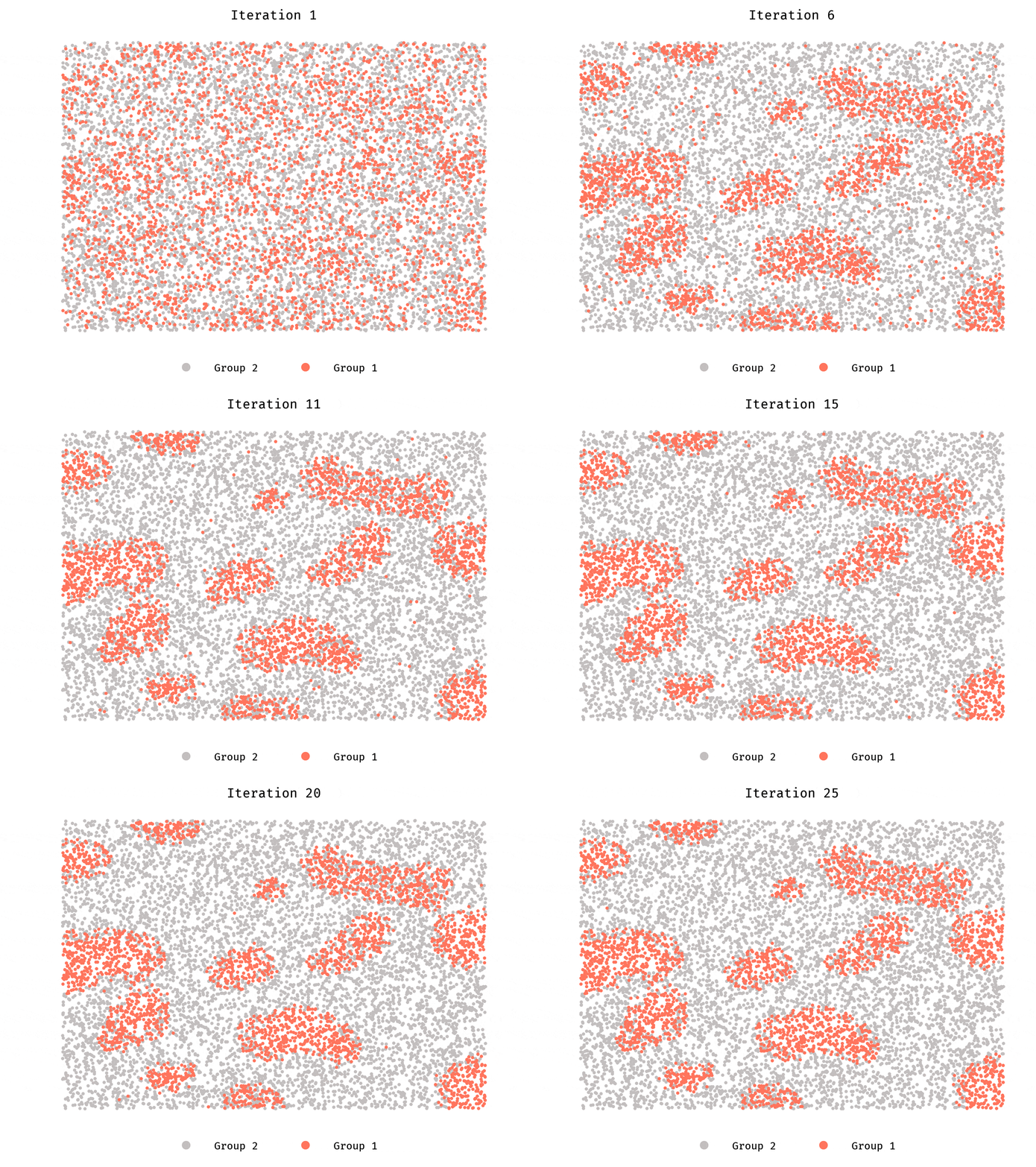
Figure 3: Population of 10k, minority group makes 30% of the population, each of agent prefers at least 33% of their neighbors to be from their own group

We still see segregation. This should not come as a surprise. The locations of the agents are drawn randomly from a uniform distribution. Agents from Group 2 are a minority (they make 30% of the population), but have a similarity preference of 33%, which means we can expect a lot of them to move in the first iterations compared to agents from Group 1 (the majority).

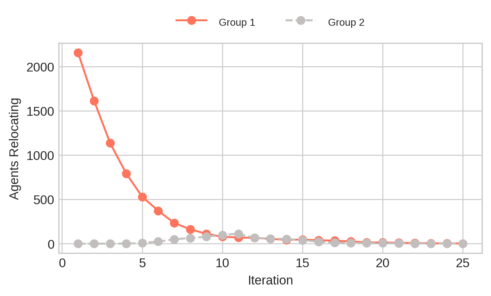
Figure 4: Number of agents relocating in each iteration by Group - Simulation 2

It stands to reason that if the similarity preference of the agents is lower than the fraction of the population the minority group represents, the initial configuration should be stable; agents won’t relocate, and neighborhoods would be well-integrated.

But is this really the case?

Simulation 3: Similarity Preference < Minority Share

Let’s consider the following initial configuration:

Neighborhood size	100
Similarity preference	0.4
Population composition	10000 agents, 2 groups (50% of population each)
Rules governing movement	If similarity preference not met, randomly relocate

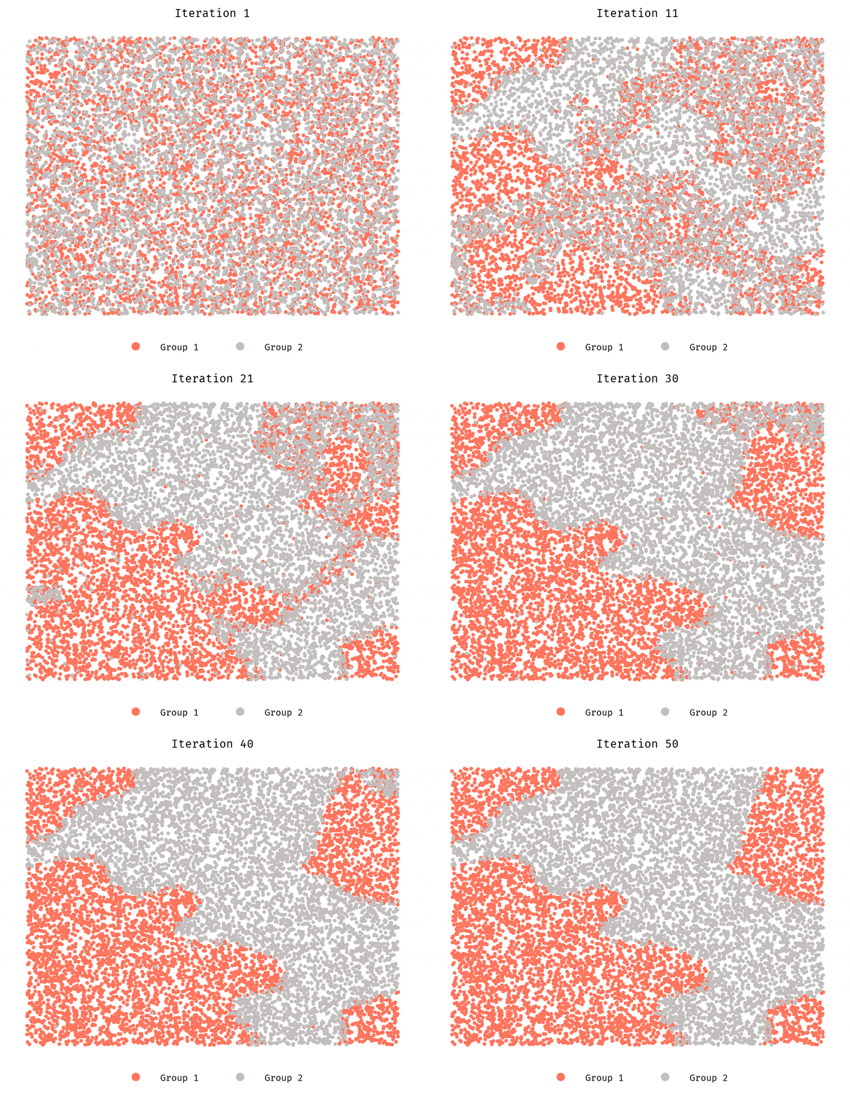
Figure 5: Agents relocating in each iteration by Group

We still see the groups segregating. Why? What’s happening here?

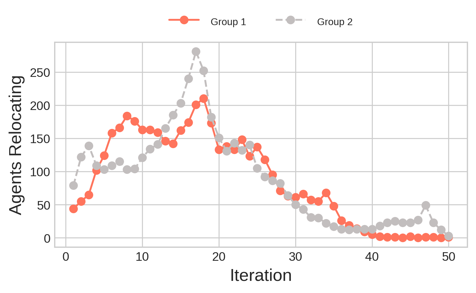
Figure 6: Number of agents relocating in each iteration by Group - Simulation 3

It has to do with how we generate the initial configuration. The initial locations are randomly drawn from a uniform distribution. Given our search space for each agent is the 100 nearest neighbors, it suffices for a few agents to be unhappy for a cascade effect to kick in and result in segregation. Randomness coupled with the low-ish number of agents simulated will still allow for initial configurations that are not stable even when the config parameters suggest they ought to.

There are a few things we can try: increase the search space to more than 100 neighbors, increase the total number of agents simulated to make probabilities play more favorably, generate the initial configuration in a less probabilistic way to enforce some guarantees, or relax the similarity preference even further compared to the minority share. All in all, we could generate initial configurations that result in integrated neighborhoods. More on this in the conclusion, but first let’s revisit a rather weak assumption regarding the rules governing the movement of agents.

Revisiting the Rules Governing Movement

Up until this point, we have assumed agents have no information on the location of other agents in the map. In real life however, information at a community level, while imperfect, exists. If you want to move, you sort of have an idea of how the neighborhood you’re moving into looks like.

Let’s equip agents with such information. One way we can do this is to create some number of guiding clusters, which at the beginning are equally spaced in the map, then agent who wants to relocate, are provided with information on each of the possible clusters they can move to: particularly the composition of those clusters (e.g. 40% Group 1, 60% Group 2.). This improves our assumption on how much information agents have on where to move, but does not say anything about the cost function of moving. For the purpose of this blog post we’ll assume the cost to move to any cluster is the same ^[5].

The Implementation does not have to be complicated. We run k-means with a predetermined number of guiding clusters (e.g. 10), then each agent before moving gets information on the composition of all clusters as well as a naive bounding space of the cluster they choose to move to (to be spawned there). For now they choose the cluster with the most favorable composition. Note that this is not perfect information. As you will see in the next section the guiding clusters are not quite the same as the segregated clusters. Think of them more like city areas.

The expected effect is a quicker process of segregation.

Simulation 4: Agents have information

We will use the same initial configuration as in Simulation 2, with the exception of the rules governing movement.

Neighborhood size	100
Similarity preference	0.333
Population composition	10000 agents, 2 groups (30% and 70% of population)
Rules governing movement	If similarity preference not met, move to cluster with most favorable representation. 7 guiding clusters.

Instead of randomly spawning to another location, each agent will now choose the most favorable guiding cluster to spawn to.

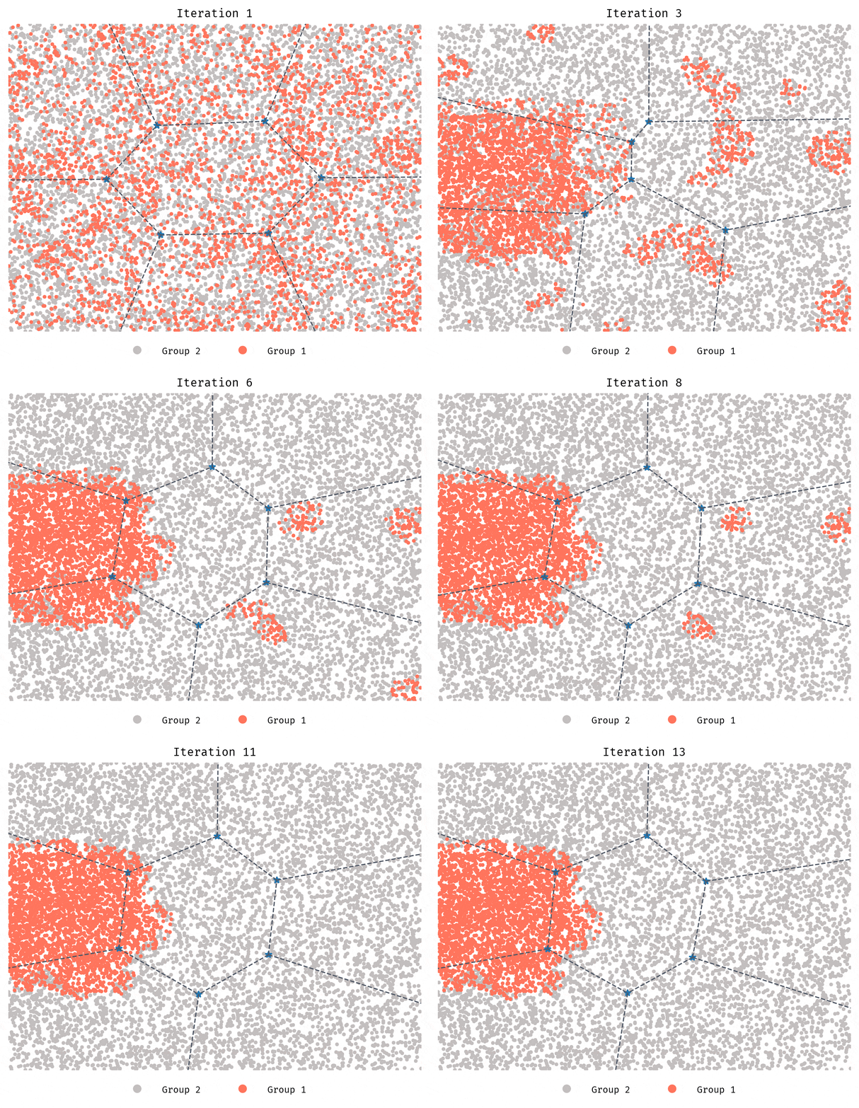
Figure 7: Population of 10k, minority group makes 30% of the population, each of agent prefers at least 33% of their neighbors to be from their own group

Unlike Simulation 2, segregation in this case is quicker and more severe.

Simulation 5: Beyond 2 groups

Neighborhood size	100
Similarity preference	0.333
Population composition	10000 agents, 3 groups (13%, 19%, and 68%)
Rules governing movement	If similarity preference not met, move to cluster with most favorable representation.

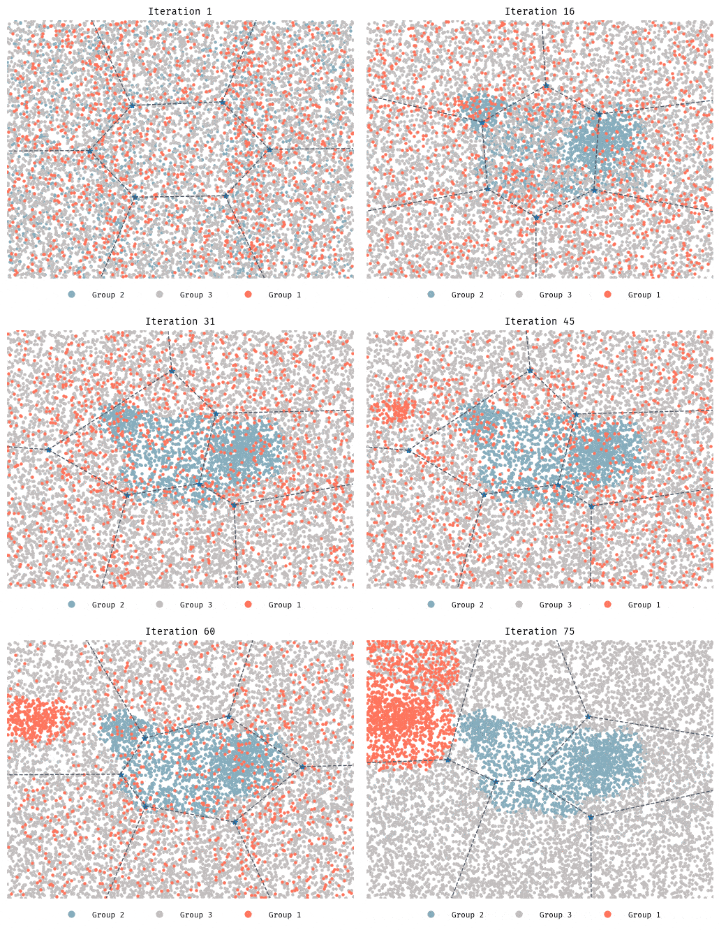
Figure 8: Population of 10k, minority group makes 30% of the population, each of agent prefers at least 33% of their neighbors to be from their own group

Although it takes longer, in this 3-group initial configuration segregation still takes place.

Final Remarks

In this blog post we built a simple simulator and looked at how collective patterns can emerge from individual behaviour. We saw how loose similarity preferences can lead to highly segregated communities based on their group membership.

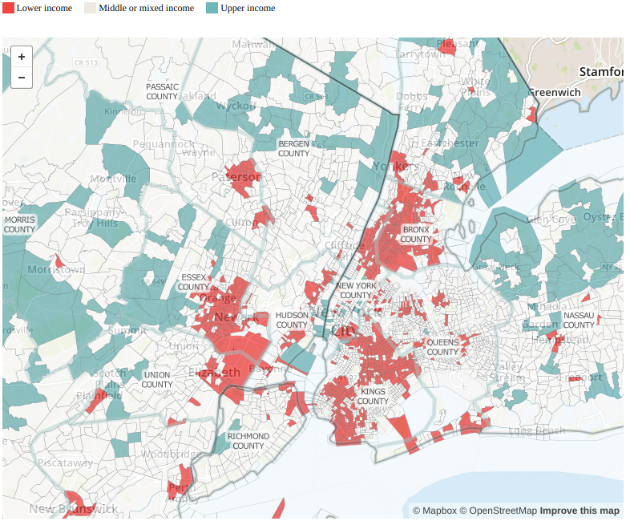
The segregation that pushed Schelling to study the issue persists today. Throughout this post I spoke about Groups because regardless of how they are defined, if group membership is a predictor of mobility in any way, simple rules result in visible segregation. Here’s an example of residential segregation by income.

Figure 9: Residential Segregation by Income in New York ^[6]

Deriving insights from this simple model suggests that as long as the similarity preference of the agents is lower than the fraction of the population the minority group represents, the initial configuration should be stable; agents won’t relocate, and neighborhoods would be well-integrated. However, we saw how very slight imbalances in the initial configuration can lead some agents to relocate and then some more and the next thing we see is complete segregation. Moreover, in reality, the similarity preference is not the only reason for people to relocate. At minimum, the similarity preference is a weighted set of preferences that may include things like income, proximity to work, employment and education opportunities etc. Any policy targeted at making our communities more integrated would have to address many of these variables.

As technologists, I wish we could do more to help domain experts (sociologists, economists, educators and policy makers at large) test assumptions, encode behaviours and ultimately recommend policy that makes our communities more integrated.

Note: The code to run the simulations is available here.

Dynamic Models of Segregation - PDF. ↩︎
Conway’s Game of Life - Wikipedia ↩︎
America is more diverse than ever — but still segregated - Washington Post ↩︎
K-D Tree - Wikipedia ↩︎
Note that this can be easily changed. For each agent that moves, we know both the current location as well as the candidate locations where the agent can relocate. This means we already have a travel distance. Next you’d need to come up with a cost function that increases with distance (e.g. linearly or exponentially). ↩︎
Residential Segregation by Income in New York - source by Pew Research Center. ↩︎